7.4 Visualizing Marker Genes on an Embedding
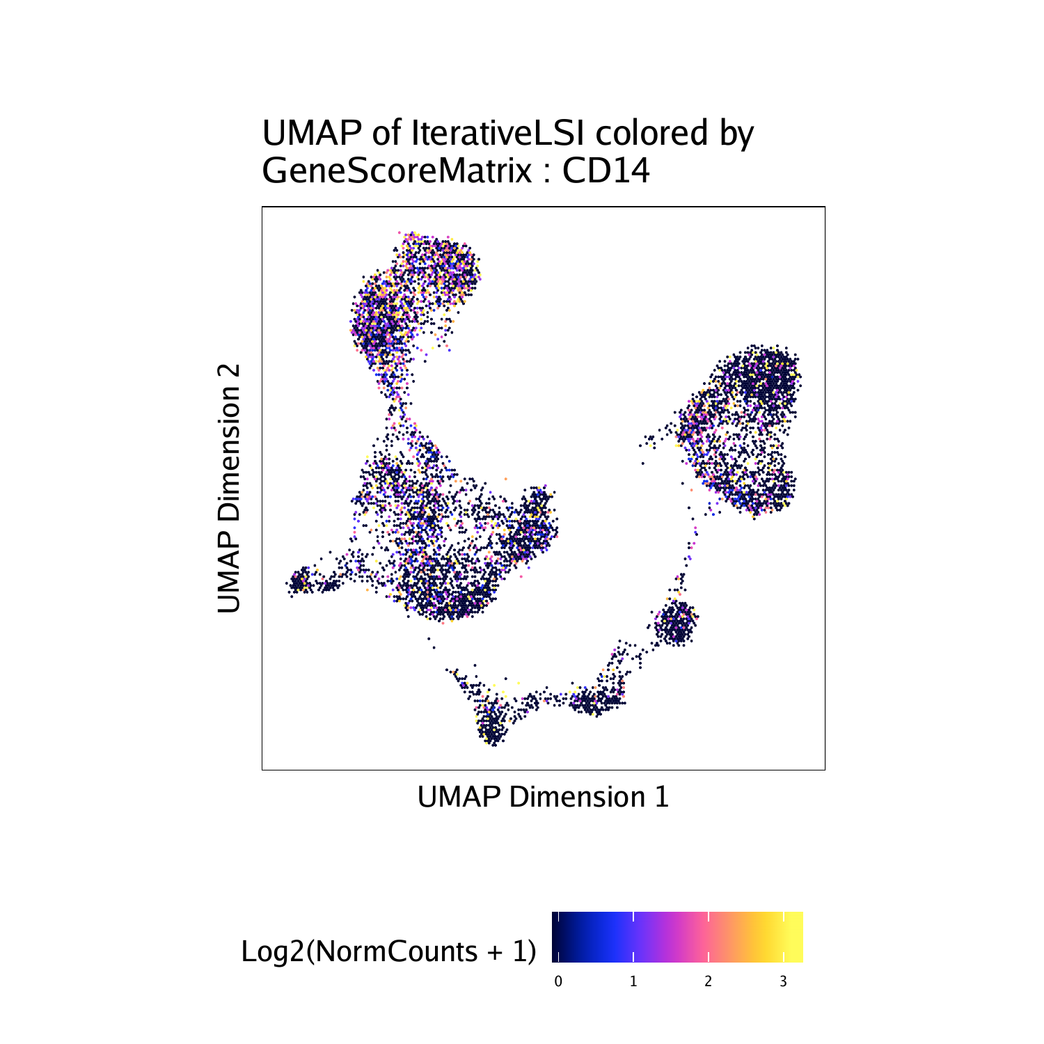
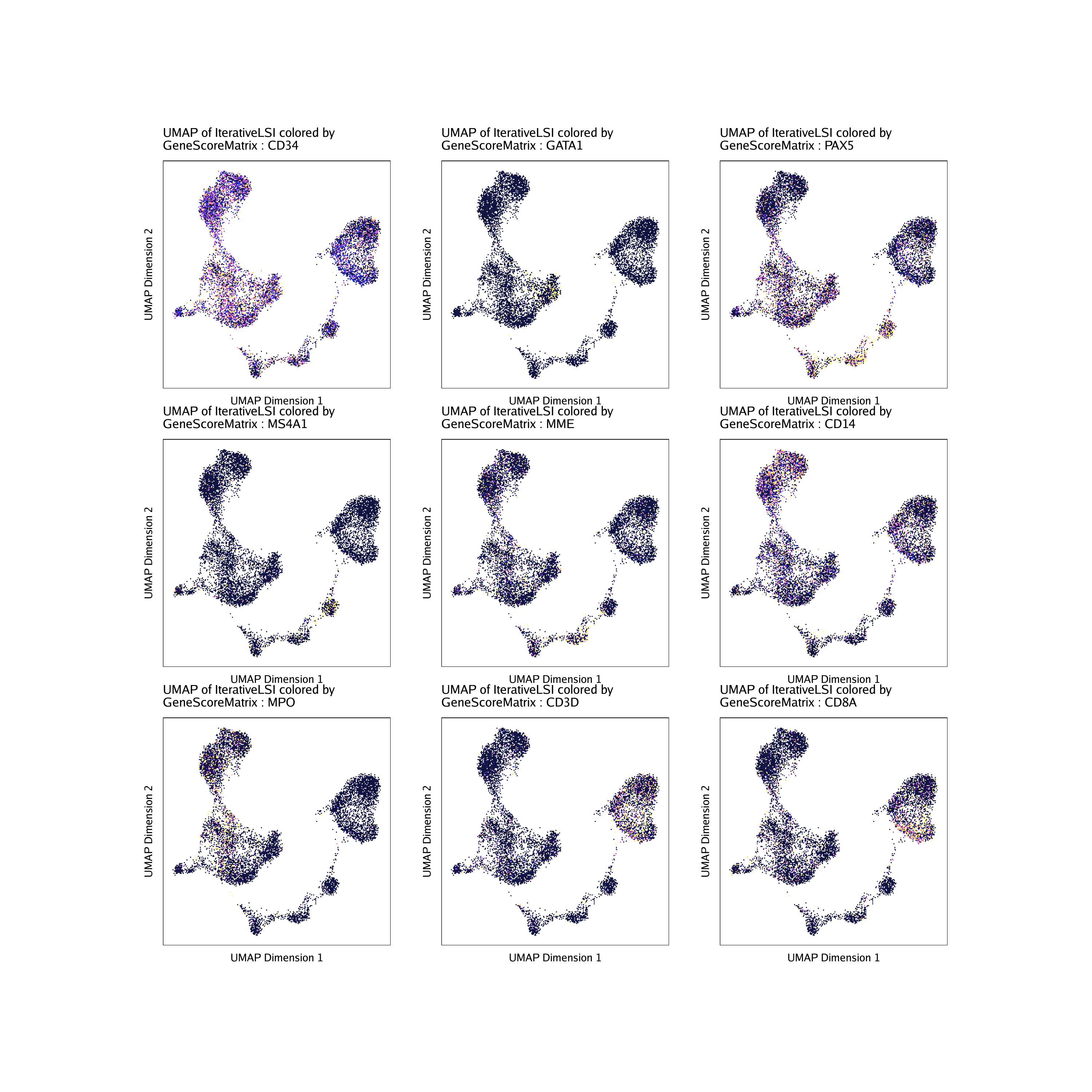
As mentioned previously, we can overlay per-cell gene scores on our UMAP embedding. This is accomplished using the colorBy and name parameters in the plotEmbedding() function.
markerGenes  <- c(
    "CD34",  #Early Progenitor
    "GATA1", #Erythroid
    "PAX5", "MS4A1", "MME", #B-Cell Trajectory
    "CD14", "MPO", #Monocytes
    "CD3D", "CD8A"#TCells
  )

p <- plotEmbedding(
    ArchRProj = projHeme2,
    colorBy = "GeneScoreMatrix",
    name = markerGenes,
    embedding = "UMAP",
    quantCut = c(0.01, 0.95),
    imputeWeights = NULL
)
## ArchR logging to : ArchRLogs/ArchR-plotEmbedding-f4e44c020f3e-Date-2020-04-15_Time-10-05-43.log
## If there is an issue, please report to github with logFile!
## Getting UMAP Embedding
## ColorBy = GeneScoreMatrix
## Getting Matrix Values…
## Getting Matrix Values…
##
## Plotting Embedding
## 1 2 3 4 5 6 7 8 9
## ArchR logging successful to : ArchRLogs/ArchR-plotEmbedding-f4e44c020f3e-Date-2020-04-15_Time-10-05-43.log
To plot a specific gene, we can subset this plot list:

To plot all genes we can use cowplot to arrange the various marker genes into a single plot.
p2 <- lapply(p, function(x){
    x + guides(color = FALSE, fill = FALSE) +
    theme_ArchR(baseSize = 6.5) +
    theme(plot.margin = unit(c(0, 0, 0, 0), "cm")) +
    theme(
        axis.text.x=element_blank(),
        axis.ticks.x=element_blank(),
        axis.text.y=element_blank(),
        axis.ticks.y=element_blank()
    )
})
do.call(cowplot::plot_grid, c(list(ncol = 3),p2))
To save an editable vectorized version of this plot, we use the plotPDF() function.
plotPDF(plotList = p,
    name = "Plot-UMAP-Marker-Genes-WO-Imputation.pdf",
    ArchRProj = projHeme2,
    addDOC = FALSE, width = 5, height = 5)
## [1] “plotting ggplot!”
## [1] “plotting ggplot!”
## [1] “plotting ggplot!”
## [1] “plotting ggplot!”
## [1] “plotting ggplot!”
## [1] “plotting ggplot!”
## [1] “plotting ggplot!”
## [1] “plotting ggplot!”
## [1] “plotting ggplot!”
## [1] 0