11.2 Plotting Marker Peaks in ArchR
ArchR provides multiple plotting functions to interact with the SummarizedExperiment objects returned by getMarkerFeatures().
11.2.1 Marker Peak Heatmaps
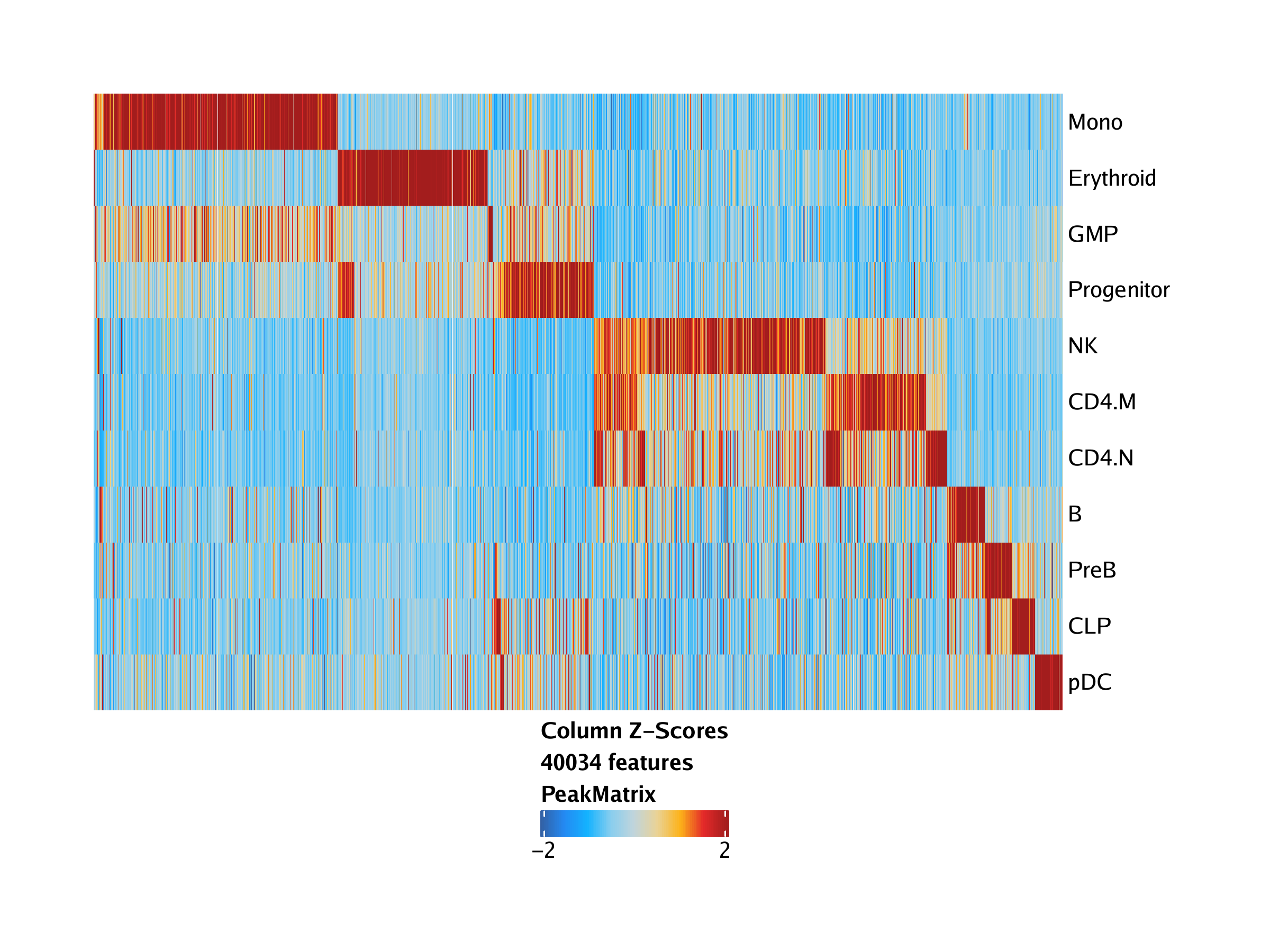
We can visualize these marker peaks (or any features output by getMarkerFeatures()) as a heatmap using the markerHeatmap() function.
heatmapPeaks <- markerHeatmap(
  seMarker = markersPeaks,
  cutOff = "FDR <= 0.1 & Log2FC >= 0.5",
  transpose = TRUE
)
## Identified 40034 markers!
## Preparing Main Heatmap..
We can plot this heatmap using draw().

To save an editable vectorized version of this plot, we use the plotPDF() function.
plotPDF(heatmapPeaks, name = "Peak-Marker-Heatmap", width = 8, height = 6, ArchRProj = projHeme5, addDOC = FALSE)## [1] 0
11.2.2 Marker Peak MA and Volcano Plots
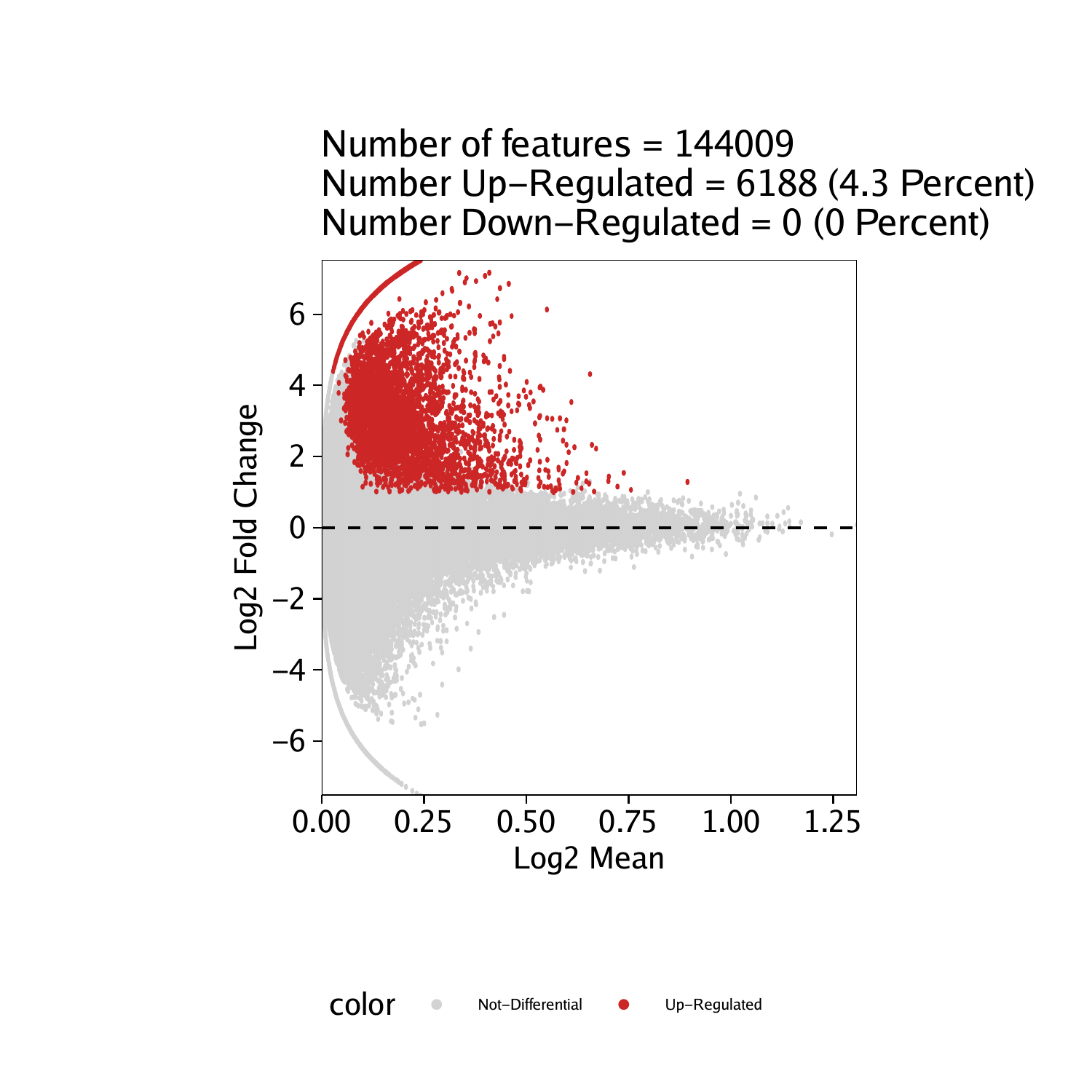
Instead of plotting a heatmap, we can also plot an MA or Volcano plot for any individual cell group. To do this, we use the markerPlot() function. For an MA plot we specify plotAs = "MA". Here we specify the “Erythroid” cell group via the name parameter.
pma <- markerPlot(seMarker = markersPeaks, name = "Erythroid", cutOff = "FDR <= 0.1 & Log2FC >= 1", plotAs = "MA")
pma
## Warning: Removed 55 rows containing missing values (geom_point_rast).

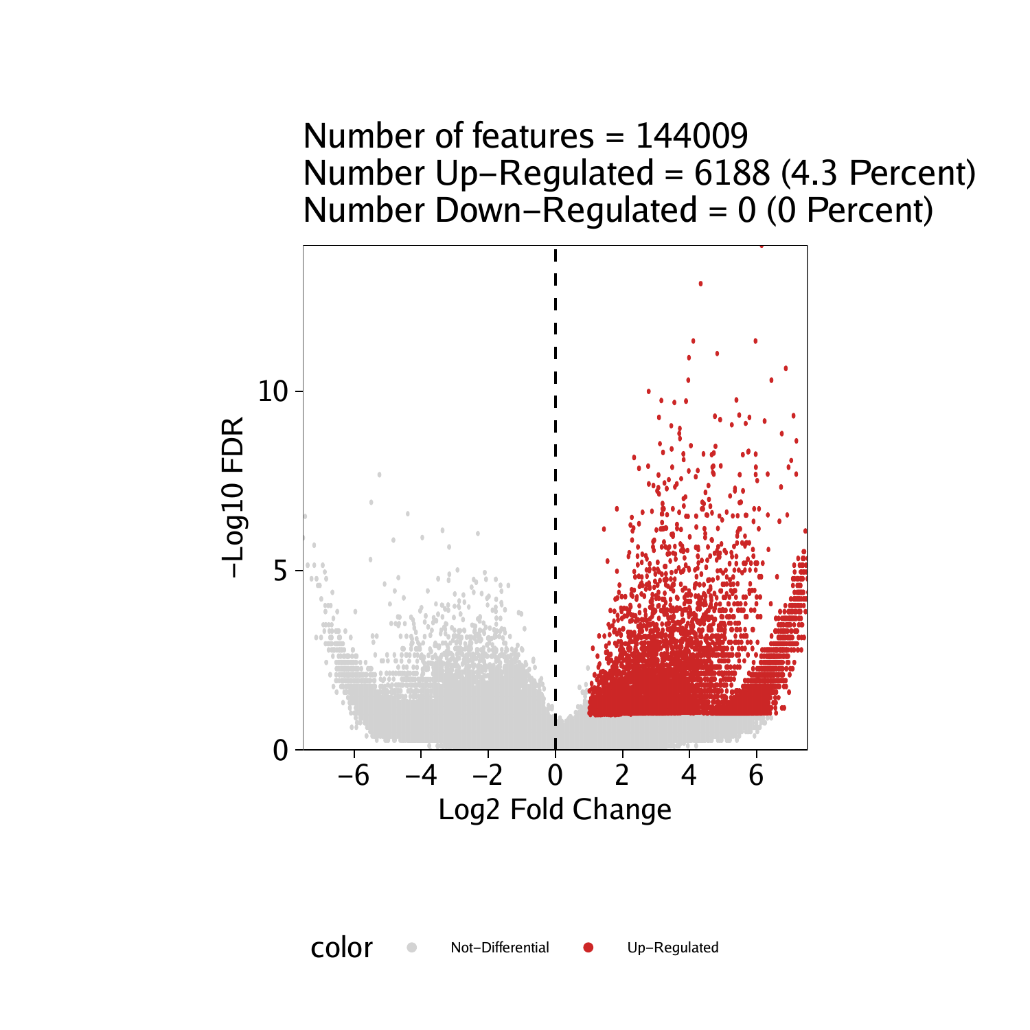
Similarly, for a Volcano plot, we specify plotAs = "Volcano".
pv <- markerPlot(seMarker = markersPeaks, name = "Erythroid", cutOff = "FDR <= 0.1 & Log2FC >= 1", plotAs = "Volcano")
pv
## Warning: Removed 55 rows containing missing values (geom_point_rast).

To save an editable vectorized version of these plots, we use the plotPDF() function.
plotPDF(pma, pv, name = "Erythroid-Markers-MA-Volcano", width = 5, height = 5, ArchRProj = projHeme5, addDOC = FALSE)## [1] “plotting ggplot!”
## Warning: Removed 55 rows containing missing values (geom_point_rast).
## Warning: Removed 55 rows containing missing values (geom_point_rast).
## [1] “plotting ggplot!”
## Warning: Removed 55 rows containing missing values (geom_point_rast).
## Warning: Removed 55 rows containing missing values (geom_point_rast).
## [1] 0
11.2.3 Marker Peaks in Browser Tracks
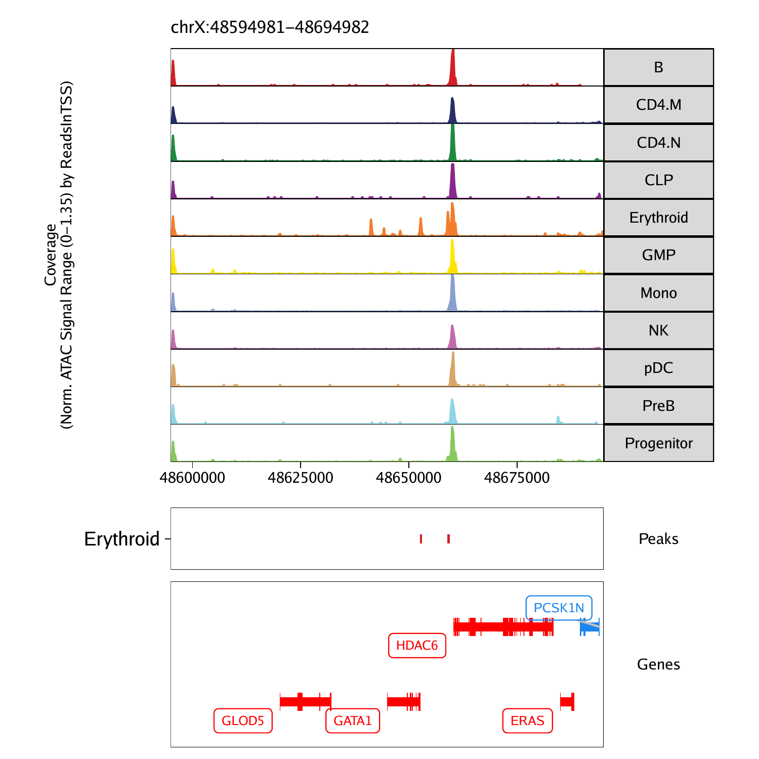
Additionally we can see these peak regions overlayed on our browser tracks by passing the relevant peak regions to the features parameterin the plotBrowserTrack() function. This will add an additional BED-style track of marker peak regions to the bottom of our ArchR track plot. Here we specify plotting the GATA1 gene via the geneSymbol parameter.
p <- plotBrowserTrack(
    ArchRProj = projHeme5,
    groupBy = "Clusters2",
    geneSymbol = c("GATA1"),
    features =  getMarkers(markersPeaks, cutOff = "FDR <= 0.1 & Log2FC >= 1", returnGR = TRUE)["Erythroid"],
    upstream = 50000,
    downstream = 50000
)
## ArchR logging to : ArchRLogs/ArchR-plotBrowserTrack-ff9f580fdbcb-Date-2020-04-15_Time-10-35-20.log
## If there is an issue, please report to github with logFile!
## Warning: ‘GenomicRangesList’ is deprecated.
## Use ‘GRangesList(…, compress=FALSE)’ instead.
## See help(“Deprecated”)
## 2020-04-15 10:35:23 : Validating Region, 0.045 mins elapsed.
## GRanges object with 1 range and 2 metadata columns:
## seqnames ranges strand | gene_id symbol
##|
## [1] chrX 48644982-48652717 + | 2623 GATA1
## ——-
## seqinfo: 24 sequences from hg19 genome
## 2020-04-15 10:35:23 : Adding Bulk Tracks (1 of 1), 0.047 mins elapsed.
## 2020-04-15 10:35:26 : Adding Feature Tracks (1 of 1), 0.095 mins elapsed.
## 2020-04-15 10:35:26 : Adding Gene Tracks (1 of 1), 0.1 mins elapsed.
## 2020-04-15 10:35:27 : Plotting, 0.109 mins elapsed.
## ArchR logging successful to : ArchRLogs/ArchR-plotBrowserTrack-ff9f580fdbcb-Date-2020-04-15_Time-10-35-20.log
We can plot this using grid::grid.draw().

To save an editable vectorized version of this plot, we use the plotPDF() function.
plotPDF(p, name = "Plot-Tracks-With-Features", width = 5, height = 5, ArchRProj = projHeme5, addDOC = FALSE)## NULL
## [1] 0