5.1 Clustering using Seurat’s FindClusters() function
We have had the most success using the graph clustering approach implemented by Seurat. In ArchR, clustering is performed using the addClusters() function which permits additional clustering parameters to be passed to the Seurat::FindClusters() function via .... In our hands, clustering using Seurat::FindClusters() is deterministic, meaning that the exact same input will always result in the exact same output.
projHeme2 <- addClusters(
    input = projHeme2,
    reducedDims = "IterativeLSI",
    method = "Seurat",
    name = "Clusters",
    resolution = 0.8
)
## ArchR logging to : ArchRLogs/ArchR-addClusters-ee735fb26d4a-Date-2020-04-15_Time-09-46-59.log
## If there is an issue, please report to github with logFile!
## 2020-04-15 09:47:08 : Running Seurats FindClusters (Stuart et al. Cell 2019), 0.142 mins elapsed.
## Computing nearest neighbor graph
## Computing SNN
## Modularity Optimizer version 1.3.0 by Ludo Waltman and Nees Jan van Eck
##
## Number of nodes: 10251
## Number of edges: 496637
##
## Running Louvain algorithm…
## Maximum modularity in 10 random starts: 0.8554
## Number of communities: 12
## Elapsed time: 1 seconds
## 2020-04-15 09:47:29 : Testing Outlier Clusters, 0.483 mins elapsed.
## 2020-04-15 09:47:29 : Assigning Cluster Names to 12 Clusters, 0.483 mins elapsed.
To access these clusters we can use the $ accessor which shows the cluster ID for each single cell.
## [1] “C3” “C8” “C4” “C3” “C11” “C3”
We can tabulate the number of cells present in each cluster:
## C1 C10 C11 C12 C2 C3 C4 C5 C6 C7 C8 C9
## 1547 879 793 1650 1085 439 351 320 387 851 1271 678
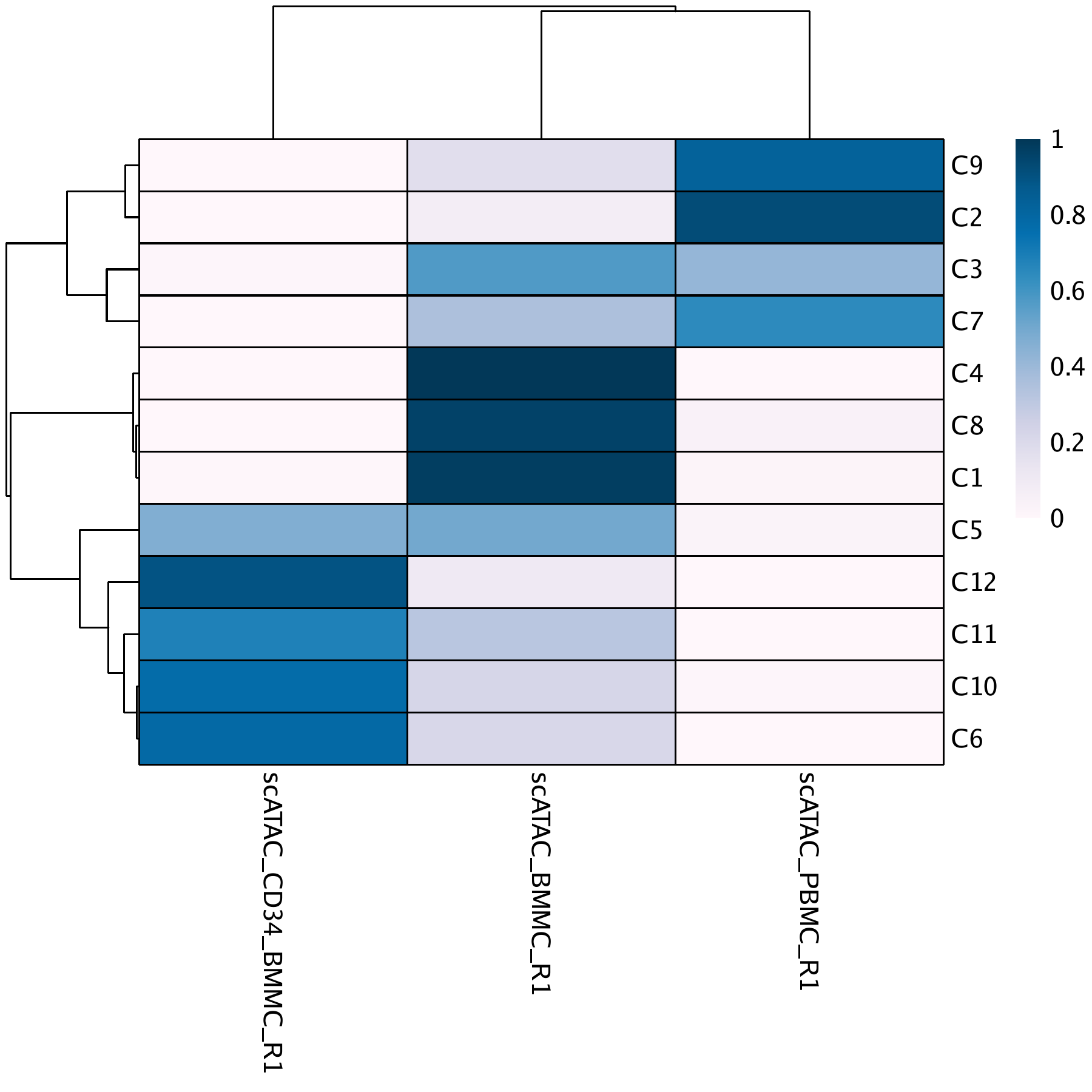
To better understand which samples reside in which clusters, we can create a cluster confusion matrix across each sample using the confusionMatrix() function.
## 12 x 3 sparse Matrix of class “dgCMatrix”
## scATAC_BMMC_R1 scATAC_CD34_BMMC_R1 scATAC_PBMC_R1
## C3 251 6 182
## C8 1219 . 52
## C4 351 . .
## C11 251 541 1
## C1 1508 9 30
## C12 172 1478 .
## C10 194 677 8
## C9 117 1 560
## C7 301 . 550
## C5 161 150 9
## C2 82 1 1002
## C6 82 305 .
To plot this confusion matrix as a heatmap, we use the pheatmap package:
library(pheatmap)
cM <- cM / Matrix::rowSums(cM)
p <- pheatmap::pheatmap(
    mat = as.matrix(cM),
    color = paletteContinuous("whiteBlue"),
    border_color = "black"
)
p
There are times where the relative location of cells within the 2-dimensional embedding does not agree perfectly with the identified clusters. More explicitly, cells from a single cluster may appear in multiple different areas of the embedding. In these contexts, it is appropriate to adjust the clustering parameters or embedding parameters until there is agreement between the two.
5.1.1 Clustering using scran
Additionally, ArchR allows for the identification of clusters with scran by changing the method parameter in addClusters().
projHeme2 <- addClusters(
    input = projHeme2,
    reducedDims = "IterativeLSI",
    method = "scran",
    name = "ScranClusters",
    k = 15
)
## ArchR logging to : ArchRLogs/ArchR-addClusters-ee735ec9887a-Date-2020-04-15_Time-09-47-32.log
## If there is an issue, please report to github with logFile!
## 2020-04-15 09:47:39 : Running Scran SNN Graph (Lun et al. F1000Res. 2016), 0.103 mins elapsed.
## 2020-04-15 09:47:49 : Identifying Clusters (Lun et al. F1000Res. 2016), 0.27 mins elapsed.
## 2020-04-15 09:50:31 : Testing Outlier Clusters, 2.98 mins elapsed.
## 2020-04-15 09:50:31 : Assigning Cluster Names to 9 Clusters, 2.98 mins elapsed.