8.3 Labeling scATAC-seq clusters with scRNA-seq information
Now that we are confident in the alignment of our scATAC-seq and scRNA-seq, we can label our scATAC-seq clusters with the cell types from our scRNA-seq data.
First, we will create a confusion matrix between our scATAC-seq clusters and the predictedGroup obtained from our integration analysis.
cM <- confusionMatrix(projHeme3$Clusters, projHeme3$predictedGroup)
labelOld <- rownames(cM)
labelOld
#  [1] "Cluster11" "Cluster2"  "Cluster12" "Cluster1"  "Cluster8"  "Cluster4"
#  [7] "Cluster9"  "Cluster5"  "Cluster7"  "Cluster14" "Cluster3"  "Cluster10"
# [13] "Cluster6"  "Cluster13"
Then, for each of our scATAC-seq clusters, we identify the cell type from predictedGroup which best defines that cluster.
Next we need to reclassify these new cluster labels to make a simpler categorization system. For each scRNA-seq cluster, we will re-define its label to something easier to interpret.
remapClust <- c(
    "01_HSC" = "Progenitor",
    "02_Early.Eryth" = "Erythroid",
    "03_Late.Eryth" = "Erythroid",
    "04_Early.Baso" = "Basophil",
    "05_CMP.LMPP" = "Progenitor",
    "06_CLP.1" = "CLP",
    "07_GMP" = "GMP",
    "08_GMP.Neut" = "GMP",
    "09_pDC" = "pDC",
    "10_cDC" = "cDC",
    "11_CD14.Mono.1" = "Mono",
    "12_CD14.Mono.2" = "Mono",
    "13_CD16.Mono" = "Mono",
    "15_CLP.2" = "CLP",
    "16_Pre.B" = "PreB",
    "17_B" = "B",
    "18_Plasma" = "Plasma",
    "19_CD8.N" = "CD8.N",
    "20_CD4.N1" = "CD4.N",
    "21_CD4.N2" = "CD4.N",
    "22_CD4.M" = "CD4.M",
    "23_CD8.EM" = "CD8.EM",
    "24_CD8.CM" = "CD8.CM",
    "25_NK" = "NK"
)
remapClust <- remapClust[names(remapClust) %in% labelNew]
Then, using the mapLabels() function, we will convert our labels to this new simpler system.
labelNew2 <- mapLabels(labelNew, oldLabels = names(remapClust), newLabels = remapClust)
labelNew2
#  [1] "GMP"        "B"          "PreB"       "CD4.N"      "Mono"
#  [6] "Erythroid"  "Progenitor" "CD4.M"      "pDC"        "NK"
# [11] "CLP"        "Mono"
Combining labelsOld and labelsNew2, we now can use the mapLabels() function again to create new cluster labels in cellColData.
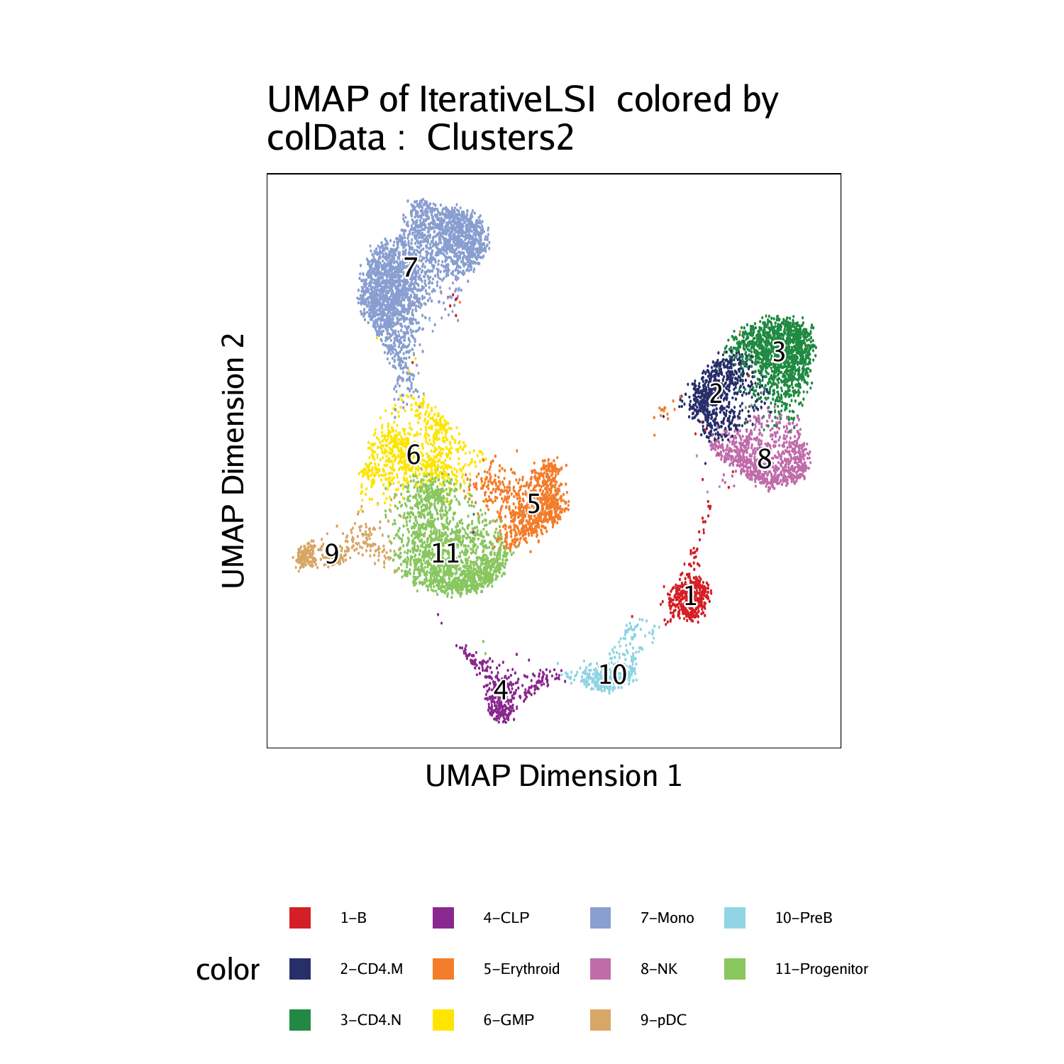
With these new labels in hand, we can plot a UMAP with the new cluster identities overlayed.
## [1] “plotting ggplot!”
## [1] 0

This paradigm can be extremely helpful when analyzing scATAC-seq data from a cellular system where scRNA-seq data already exists. As mentioned previously, this integration of scATAC-seq with scRNA-seq also provides a beautiful framework for more complex gene regulation analyses that will be described in later chapters.
To save an editable vectorized version of this plot, we use the plotPDF() function.
plotPDF(p1, name = "Plot-UMAP-Remap-Clusters.pdf", ArchRProj = projHeme2, addDOC = FALSE, width = 5, height = 5)We can now save our original projHeme3 using saveArchRProject from ArchR.
## Copying ArchRProject to new outputDirectory : /oak/stanford/groups/howchang/users/jgranja/ArchRTutorial/ArchRBook/BookOutput4/Save-ProjHeme3
## Copying Arrow Files…
## Copying Arrow Files (1 of 3)
## Copying Arrow Files (2 of 3)
## Copying Arrow Files (3 of 3)
## Getting ImputeWeights
## Dropping ImputeWeights…
## Copying Other Files…
## Copying Other Files (1 of 4): Embeddings
## Copying Other Files (2 of 4): IterativeLSI
## Copying Other Files (3 of 4): IterativeLSI2
## Copying Other Files (4 of 4): Plots
## Saving ArchRProject…