13.1 Motif Deviations

First, lets make sure we have added motif annotations to our ArchRProject.

if("Motif" %ni% names(projHeme5@peakAnnotation)){
    projHeme5 <- addMotifAnnotations(ArchRProj = projHeme5, motifSet = "cisbp", name = "Motif")
}

We also need to add a set of background peaks which are used in computing deviations. Background peaks are chosen using the chromVAR::getBackgroundPeaks() function which samples peaks based on similarity in GC-content and number of fragments across all samples using the Mahalanobis distance.

projHeme5 <- addBgdPeaks(projHeme5)

## Identifying Background Peaks!
## No methods found in package ‘IRanges’ for request: ‘score’ when loading ‘TFBSTools’

We are now ready to compute per-cell deviations accross all of our motif annotations using the addDeviationsMatrix() function. This function has an optional parameter called matrixName that allows us to define the name of the deviations matrix that will be stored in the Arrow files. If we do not provide a value to this parameter, as in the example below, this function creates a matrix name by adding the word “Matrix” to the name of the peakAnnotation. The example below creates a deviations matrix in each of our Arrow files called “MotifMatrix”.

projHeme5 <- addDeviationsMatrix(
  ArchRProj = projHeme5, 
  peakAnnotation = "Motif",
  force = TRUE
)

## Using Previous Background Peaks!
## ArchR logging to : ArchRLogs/ArchR-addDeviationsMatrix-103741bce39ff-Date-2020-04-15_Time-10-45-35.log
## If there is an issue, please report to github with logFile!
## NULL
## 2020-04-15 10:45:40 : Batch Execution w/ safelapply!, 0 mins elapsed.
## ###########
## 2020-04-15 10:57:19 : Completed Computing Deviations!, 11.734 mins elapsed.
## ###########
## ArchR logging successful to : ArchRLogs/ArchR-addDeviationsMatrix-103741bce39ff-Date-2020-04-15_Time-10-45-35.log

To access these deviations, we use the getVarDeviations() function. If we want this function to return a ggplot object, we set plot = TRUE otherwise, this function would return the DataFrame object. The head of that DataFrame object is displayed by default when the function is run.

plotVarDev <- getVarDeviations(projHeme5, name = "MotifMatrix", plot = TRUE)

## DataFrame with 6 rows and 6 columns
## seqnames idx name combinedVars combinedMeans
##
## f388 z 388 GATA2_388 11.9292478607949 -0.034894792575792
## f155 z 155 CEBPA_155 11.8070700579364 -0.174087405321135
## f383 z 383 GATA1_383 11.8045825337775 -0.0378306234562619
## f336 z 336 SPIB_336 11.3432739583017 -0.0819836042460723
## f385 z 385 GATA5_385 10.8828679211543 -0.036867577013264
## f651 z 651 SMARCC1_651 10.2885493109675 -0.131812047523969
## rank
##
## f388 1
## f155 2
## f383 3
## f336 4
## f385 5
## f651 6

From the above snapshot of the DataFrame, you can see that the seqnames of the MotifMatrix are not chromosomes. Typically, in matrices like the TileMatrix, PeakMatrix, and GeneScoreMatrix, we store the chromosome information in seqnames. The MotifMatrix does not have any corresponding position information but, instead, stores both the “devations” and “z-scores” from chromVAR into the same matrix using two different seqnames - deviations and z. This becomes important later on if you try to use the MotifMatrix (which is of class Sparse.Assays.Matrix) in functions such as getMarkerFeatures(). In these types of operations, ArchR will expect you to subset MotifMatrix to one of the two seqnames (i.e. select either z-scores or deviations to perform calculations).

We can then plot these variable deviations.

plotVarDev

## Warning: Removed 1 rows containing missing values (geom_point).

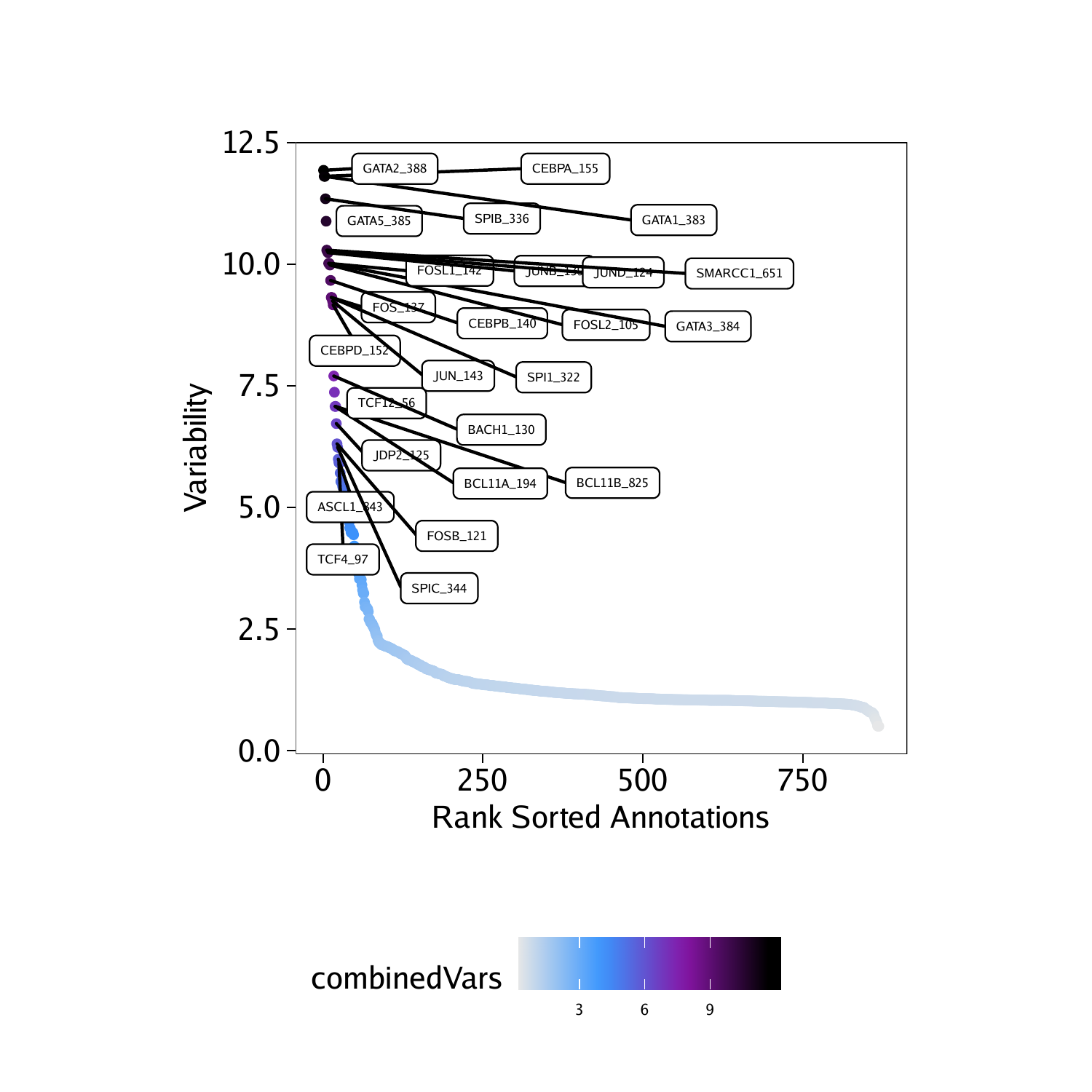
To save an editable vectorized version of this plot, we use the plotPDF() function.

plotPDF(plotVarDev, name = "Variable-Motif-Deviation-Scores", width = 5, height = 5, ArchRProj = projHeme5, addDOC = FALSE)

## [1] “plotting ggplot!”
## Warning: Removed 1 rows containing missing values (geom_point).
## Warning: Removed 1 rows containing missing values (geom_point).
## [1] 0

What if we want to extract a subset of motifs for downstream analysis? We can do this using the getFeatures() function. The paste(motifs, collapse="|") statement below creates a concatenated or statement that enables selection of all of the motifs.

motifs <- c("GATA1", "CEBPA", "EBF1", "IRF4", "TBX21", "PAX5")
markerMotifs <- getFeatures(projHeme5, select = paste(motifs, collapse="|"), useMatrix = "MotifMatrix")
markerMotifs

## [1] “z:TBX21_780” “z:PAX5_709” “z:IRF4_632”
## [4] “z:GATA1_383” “z:CEBPA_155” “z:EBF1_67”
## [7] “z:SREBF1_22” “deviations:TBX21_780” “deviations:PAX5_709”
## [10] “deviations:IRF4_632” “deviations:GATA1_383” “deviations:CEBPA_155”
## [13] “deviations:EBF1_67” “deviations:SREBF1_22”

As mentioned above, MotifMatrix contains seqnames for both z-scores and deviations, shown above by “z:” and “deviations:”. To get just the features corresponding to z-scores, we can use grep. Unfortunately, in the example motifs shown above, you can see that in addition to “EBF1”, we also selected “SREBF1” which we do not want to analyze. Because of this, we remove it below using the %ni% expression which is an ArchR helper function that provides the opposite of %in% from base R.

markerMotifs <- grep("z:", markerMotifs, value = TRUE)
markerMotifs <- markerMotifs[markerMotifs %ni% "z:SREBF1_22"]
markerMotifs

## [1] “z:TBX21_780” “z:PAX5_709” “z:IRF4_632” “z:GATA1_383” “z:CEBPA_155”
## [6] “z:EBF1_67”

Now that we have the names of the features that we are interested in, we can plot the distribution of chromVAR deviation scores for each cluster. Notice that we supply the impute weights that we calculated previously during our gene score analyses. As a reminder, these impute weights allow us to smooth the signal across nearby cells which is helpful in the context of our sparse scATAC-seq data.

p <- plotGroups(ArchRProj = projHeme5, 
  groupBy = "Clusters2", 
  colorBy = "MotifMatrix", 
  name = markerMotifs,
  imputeWeights = getImputeWeights(projHeme5)
)

## Getting ImputeWeights
## Getting Matrix Values…
## Getting Matrix Values…
##
## ArchR logging to : ArchRLogs/ArchR-imputeMatrix-103746efc5207-Date-2020-04-15_Time-10-57-40.log
## If there is an issue, please report to github with logFile!
## Using weights on disk
## Using weights on disk
## 1 2 3 4 5 6

We can use cowplot to plot the distributions of all of these motifs in a single plot.

p2 <- lapply(seq_along(p), function(x){
  if(x != 1){
    p[[x]] + guides(color = FALSE, fill = FALSE) + 
    theme_ArchR(baseSize = 6) +
    theme(plot.margin = unit(c(0.1, 0.1, 0.1, 0.1), "cm")) +
    theme(
        axis.text.y=element_blank(), 
        axis.ticks.y=element_blank(),
        axis.title.y=element_blank()
    ) + ylab("")
  }else{
    p[[x]] + guides(color = FALSE, fill = FALSE) + 
    theme_ArchR(baseSize = 6) +
    theme(plot.margin = unit(c(0.1, 0.1, 0.1, 0.1), "cm")) +
    theme(
        axis.ticks.y=element_blank(),
        axis.title.y=element_blank()
    ) + ylab("")
  }
})
do.call(cowplot::plot_grid, c(list(nrow = 1, rel_widths = c(2, rep(1, length(p2) - 1))),p2))

## Picking joint bandwidth of 0.0181
## Picking joint bandwidth of 0.02
## Picking joint bandwidth of 0.07
## Picking joint bandwidth of 0.109
## Picking joint bandwidth of 0.102
## Picking joint bandwidth of 0.0703

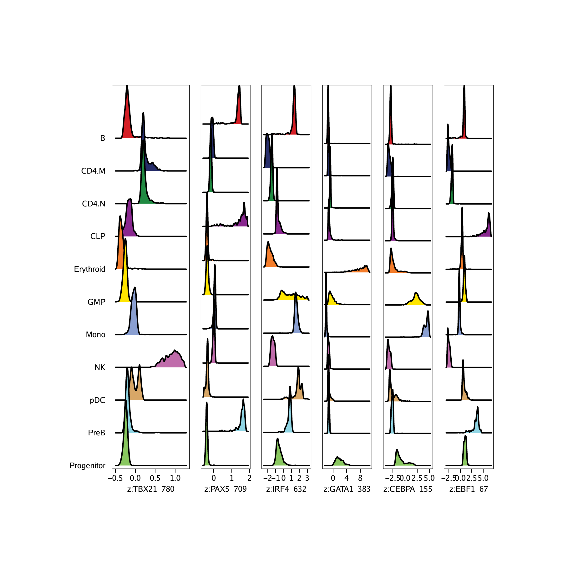
To save an editable vectorized version of this plot, we use the plotPDF() function.

plotPDF(p, name = "Plot-Groups-Deviations-w-Imputation", width = 5, height = 5, ArchRProj = projHeme5, addDOC = FALSE)

## [1] “plotting ggplot!”
## Picking joint bandwidth of 0.0181
## Picking joint bandwidth of 0.0181
## [1] “plotting ggplot!”
## Picking joint bandwidth of 0.02
## Picking joint bandwidth of 0.02
## [1] “plotting ggplot!”
## Picking joint bandwidth of 0.07
## Picking joint bandwidth of 0.07
## [1] “plotting ggplot!”
## Picking joint bandwidth of 0.109
## Picking joint bandwidth of 0.109
## [1] “plotting ggplot!”
## Picking joint bandwidth of 0.102
## Picking joint bandwidth of 0.102
## [1] “plotting ggplot!”
## Picking joint bandwidth of 0.0703
## Picking joint bandwidth of 0.0703
## [1] 0

Instead of looking at the distributions of these z-scores, we can overlay the z-scores on our UMAP embedding as we’ve done previously for gene scores.

p <- plotEmbedding(
    ArchRProj = projHeme5, 
    colorBy = "MotifMatrix", 
    name = sort(markerMotifs), 
    embedding = "UMAP",
    imputeWeights = getImputeWeights(projHeme5)
)

## Getting ImputeWeights
## ArchR logging to : ArchRLogs/ArchR-plotEmbedding-10374bec190f-Date-2020-04-15_Time-10-58-03.log
## If there is an issue, please report to github with logFile!
## Getting UMAP Embedding
## ColorBy = MotifMatrix
## Getting Matrix Values…
## Getting Matrix Values…
##
## Imputing Matrix
## Using weights on disk
## Using weights on disk
## Plotting Embedding
## 1 2 3 4 5 6
## ArchR logging successful to : ArchRLogs/ArchR-plotEmbedding-10374bec190f-Date-2020-04-15_Time-10-58-03.log

We can plot all of these motif UMAPs using cowplot.

p2 <- lapply(p, function(x){
    x + guides(color = FALSE, fill = FALSE) + 
    theme_ArchR(baseSize = 6.5) +
    theme(plot.margin = unit(c(0, 0, 0, 0), "cm")) +
    theme(
        axis.text.x=element_blank(), 
        axis.ticks.x=element_blank(), 
        axis.text.y=element_blank(), 
        axis.ticks.y=element_blank()
    )
})
do.call(cowplot::plot_grid, c(list(ncol = 3),p2))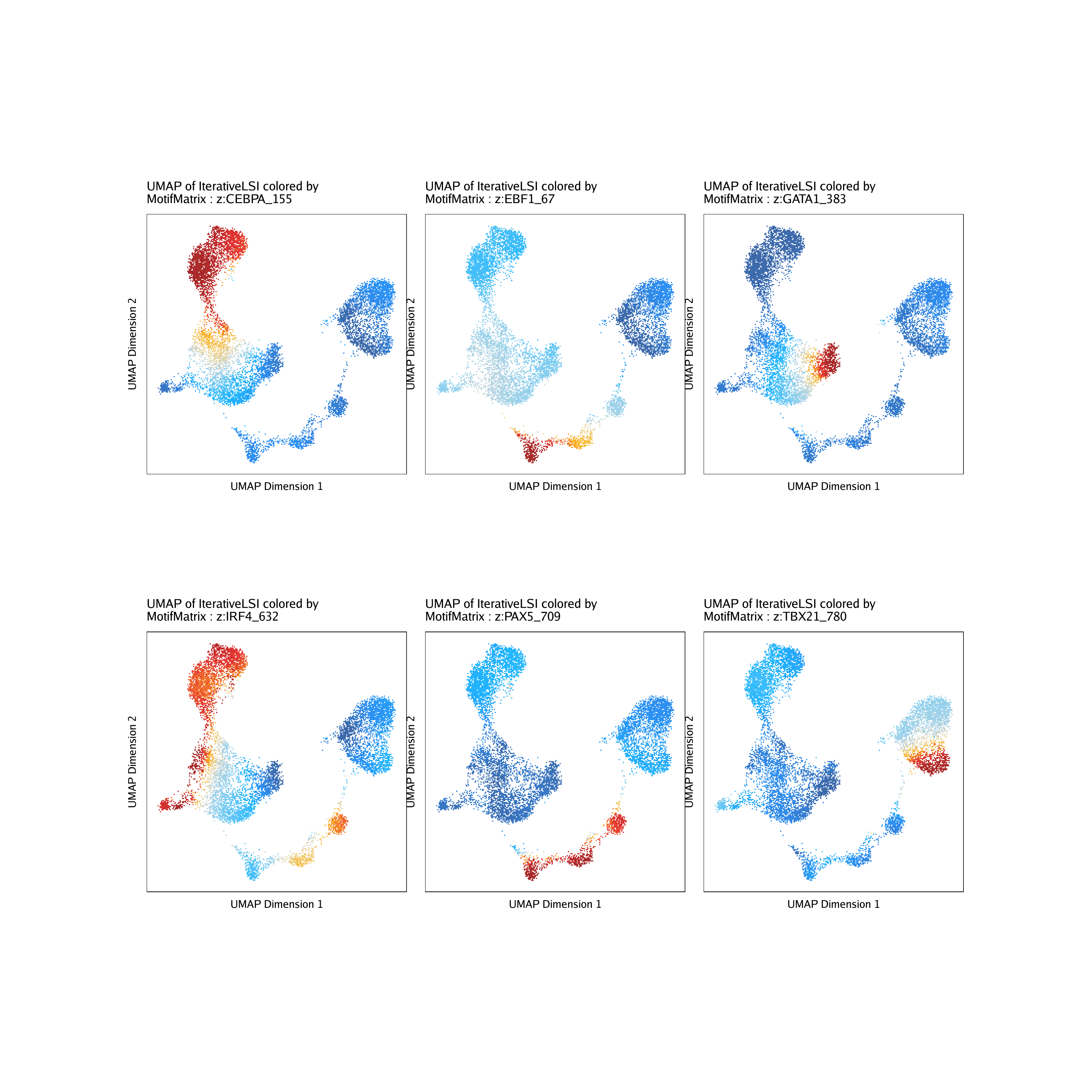

To see how these TF deviation z-scores compare to the inferred gene expression via gene scores of the corresponding TF genes, we can overlay the gene scores for each of these TFs on the UMAP embedding.

markerRNA <- getFeatures(projHeme5, select = paste(motifs, collapse="|"), useMatrix = "GeneScoreMatrix")
markerRNA <- markerRNA[markerRNA %ni% c("SREBF1","CEBPA-DT")]
markerRNA

## [1] “TBX21” “CEBPA” “EBF1” “IRF4” “PAX5” “GATA1”

p <- plotEmbedding(
    ArchRProj = projHeme5, 
    colorBy = "GeneScoreMatrix", 
    name = sort(markerRNA), 
    embedding = "UMAP",
    imputeWeights = getImputeWeights(projHeme5)
)

## Getting ImputeWeights
## ArchR logging to : ArchRLogs/ArchR-plotEmbedding-1037475e6dc52-Date-2020-04-15_Time-10-58-30.log
## If there is an issue, please report to github with logFile!
## Getting UMAP Embedding
## ColorBy = GeneScoreMatrix
## Getting Matrix Values…
## Getting Matrix Values…
##
## Imputing Matrix
## Using weights on disk
## Using weights on disk
## Plotting Embedding
## 1 2 3 4 5 6
## ArchR logging successful to : ArchRLogs/ArchR-plotEmbedding-1037475e6dc52-Date-2020-04-15_Time-10-58-30.log

p2 <- lapply(p, function(x){
    x + guides(color = FALSE, fill = FALSE) + 
    theme_ArchR(baseSize = 6.5) +
    theme(plot.margin = unit(c(0, 0, 0, 0), "cm")) +
    theme(
        axis.text.x=element_blank(), 
        axis.ticks.x=element_blank(), 
        axis.text.y=element_blank(), 
        axis.ticks.y=element_blank()
    )
})
do.call(cowplot::plot_grid, c(list(ncol = 3),p2))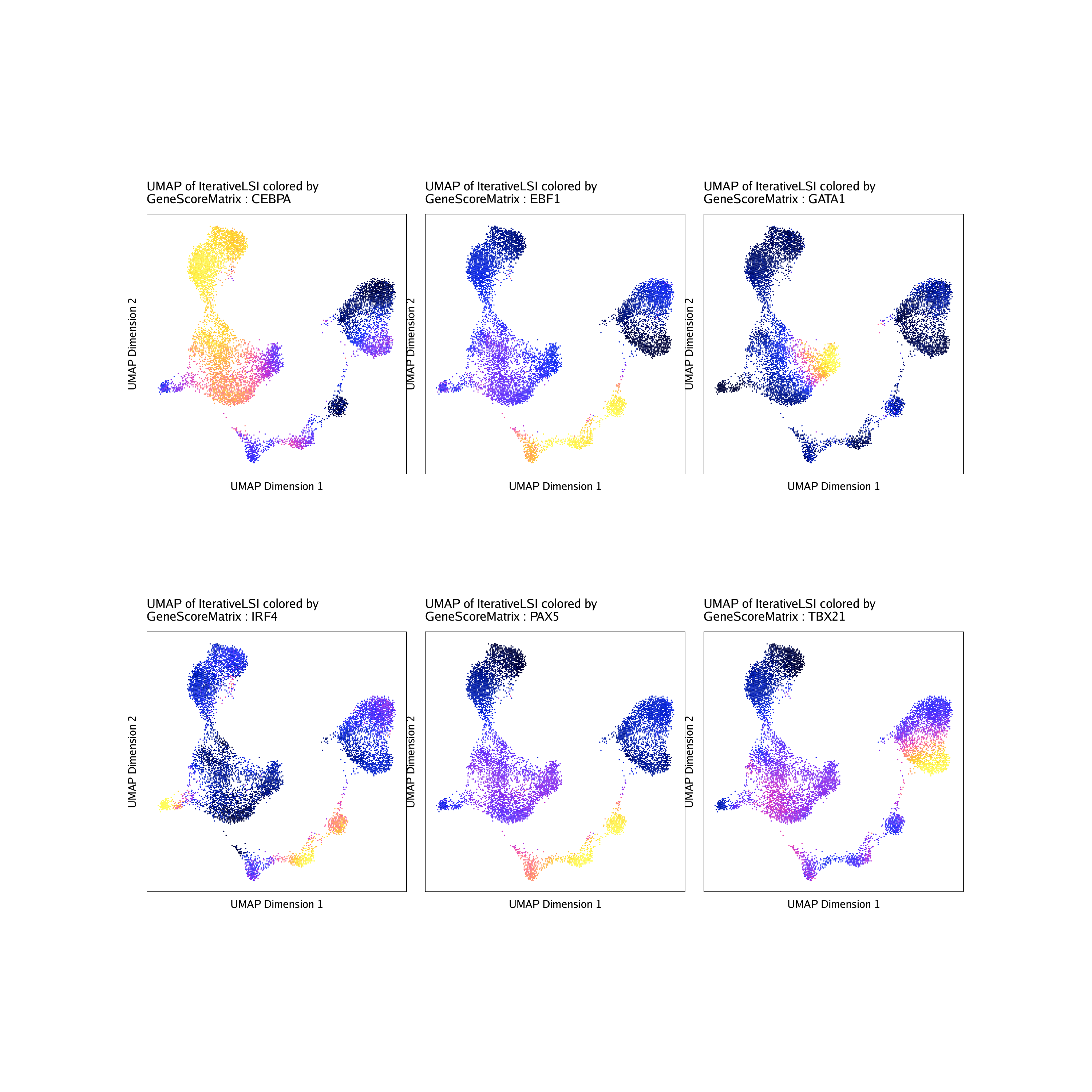

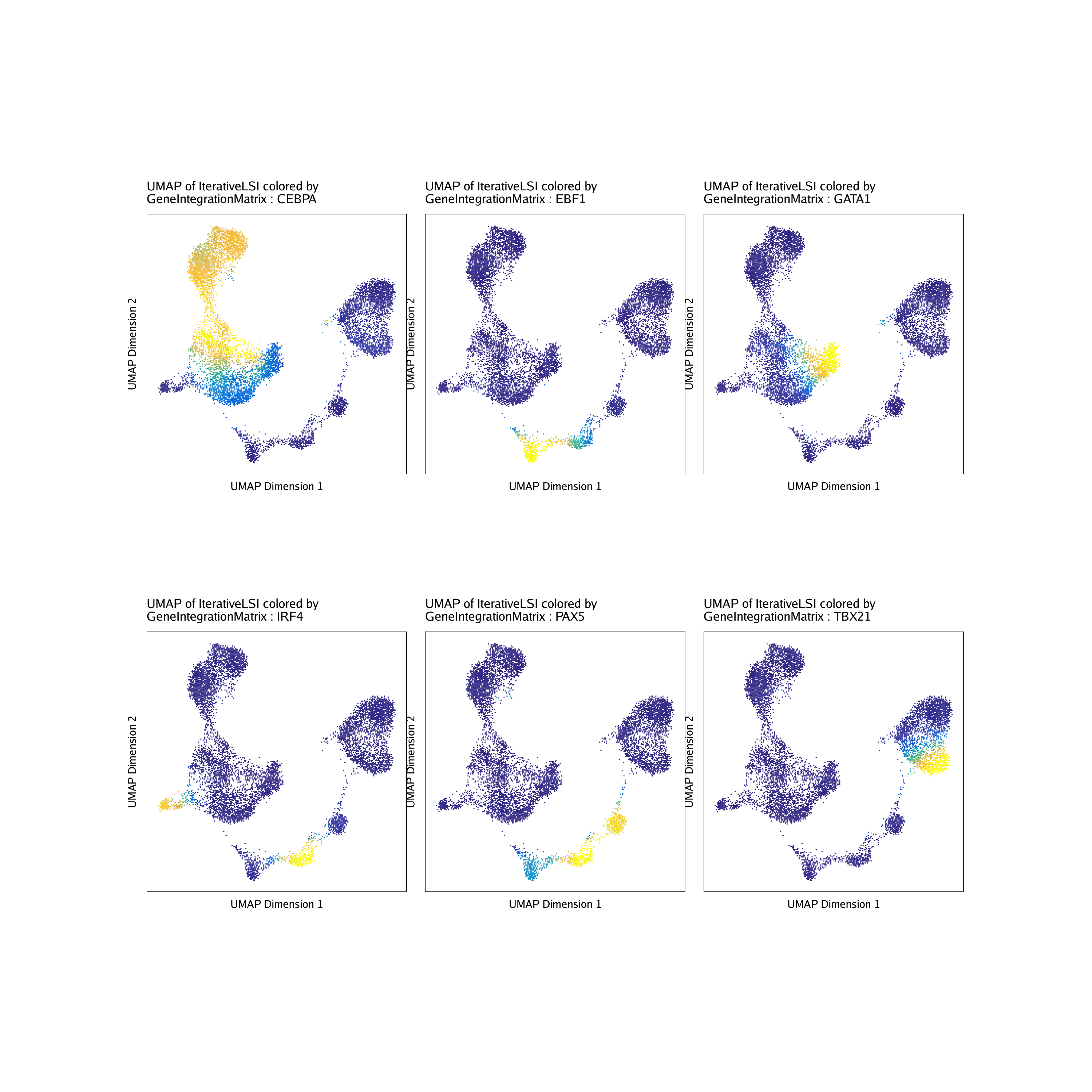
Similarly, because we previously linked our scATAC-seq data with corresponding scRNA-seq data, we can plot the linked gene expression for each of these TFs on the UMAP embedding.

markerRNA <- getFeatures(projHeme5, select = paste(motifs, collapse="|"), useMatrix = "GeneIntegrationMatrix")
markerRNA <- markerRNA[markerRNA %ni% c("SREBF1","CEBPA-DT")]
markerRNA

## [1] “TBX21” “CEBPA” “EBF1” “IRF4” “PAX5” “GATA1”

p <- plotEmbedding(
    ArchRProj = projHeme5, 
    colorBy = "GeneIntegrationMatrix", 
    name = sort(markerRNA), 
    embedding = "UMAP",
    continuousSet = "blueYellow",
    imputeWeights = getImputeWeights(projHeme5)
)

## Getting ImputeWeights
## ArchR logging to : ArchRLogs/ArchR-plotEmbedding-10374438d3144-Date-2020-04-15_Time-10-58-56.log
## If there is an issue, please report to github with logFile!
## Getting UMAP Embedding
## ColorBy = GeneIntegrationMatrix
## Getting Matrix Values…
## Getting Matrix Values…
##
## Imputing Matrix
## Using weights on disk
## Using weights on disk
## Plotting Embedding
## 1 2 3 4 5 6
## ArchR logging successful to : ArchRLogs/ArchR-plotEmbedding-10374438d3144-Date-2020-04-15_Time-10-58-56.log

p2 <- lapply(p, function(x){
    x + guides(color = FALSE, fill = FALSE) + 
    theme_ArchR(baseSize = 6.5) +
    theme(plot.margin = unit(c(0, 0, 0, 0), "cm")) +
    theme(
        axis.text.x=element_blank(), 
        axis.ticks.x=element_blank(), 
        axis.text.y=element_blank(), 
        axis.ticks.y=element_blank()
    )
})
do.call(cowplot::plot_grid, c(list(ncol = 3),p2))