8.2 Adding Pseudo-scRNA-seq profiles for each scATAC-seq cell
Now that we are satisfied with the results of our scATAC-seq and scRNA-seq integration, we can re-run the integration with addToArrow = TRUE to add the linked gene expression data to each of the Arrow files. As described previously, we pass the groupList to constrain the integration and column names to nameCell, nameGroup, and nameScore for each of the metadata columns we will add to cellColData. Here, we create projHeme3 which will be carried forward in the tutorial.
#~5 minutes
projHeme3 <- addGeneIntegrationMatrix(
    ArchRProj = projHeme2,
    useMatrix = "GeneScoreMatrix",
    matrixName = "GeneIntegrationMatrix",
    reducedDims = "IterativeLSI",
    seRNA = seRNA,
    addToArrow = TRUE,
    force= TRUE,
    groupList = groupList,
    groupRNA = "BioClassification",
    nameCell = "predictedCell",
    nameGroup = "predictedGroup",
    nameScore = "predictedScore"
)
## ArchR logging to : ArchRLogs/ArchR-addGeneIntegrationMatrix-f66317d3557e-Date-2020-04-15_Time-10-16-26.log
## If there is an issue, please report to github with logFile!
## 2020-04-15 10:16:26 : Running Seurat’s Integration Stuart* et al 2019, 0.009 mins elapsed.
## 2020-04-15 10:16:27 : Checking ATAC Input, 0.021 mins elapsed.
## 2020-04-15 10:16:27 : Checking RNA Input, 0.021 mins elapsed.
## 2020-04-15 10:16:38 : Creating Integration Blocks, 0.211 mins elapsed.
## 2020-04-15 10:16:39 : Prepping Interation Data, 0.215 mins elapsed.
## 2020-04-15 10:16:39 : Computing Integration in 2 Integration Blocks!, 0 mins elapsed.
## 2020-04-15 10:19:30 : Transferring Data to ArrowFiles, 2.843 mins elapsed.
## 2020-04-15 10:20:47 : Completed Integration with RNA Matrix, 4.133 mins elapsed.
## ArchR logging successful to : ArchRLogs/ArchR-addGeneIntegrationMatrix-f66317d3557e-Date-2020-04-15_Time-10-16-26.log
Now, when we check which matrices are available using getAvailableMatrices(), we see that the GeneIntegrationMatrix has been added to the Arrow files.
## [1] “GeneIntegrationMatrix” “GeneScoreMatrix” “TileMatrix”
With this new GeneIntegrationMatrix we can compare the linked gene expression with the inferred gene expression obtained through gene scores.
First, lets make sure we have added impute weights to our project:
## 2020-04-15 10:20:49 : Computing Impute Weights Using Magic (Cell 2018), 0 mins elapsed.
## 2020-04-15 10:20:59 : Completed Getting Magic Weights!, 0.176 mins elapsed.
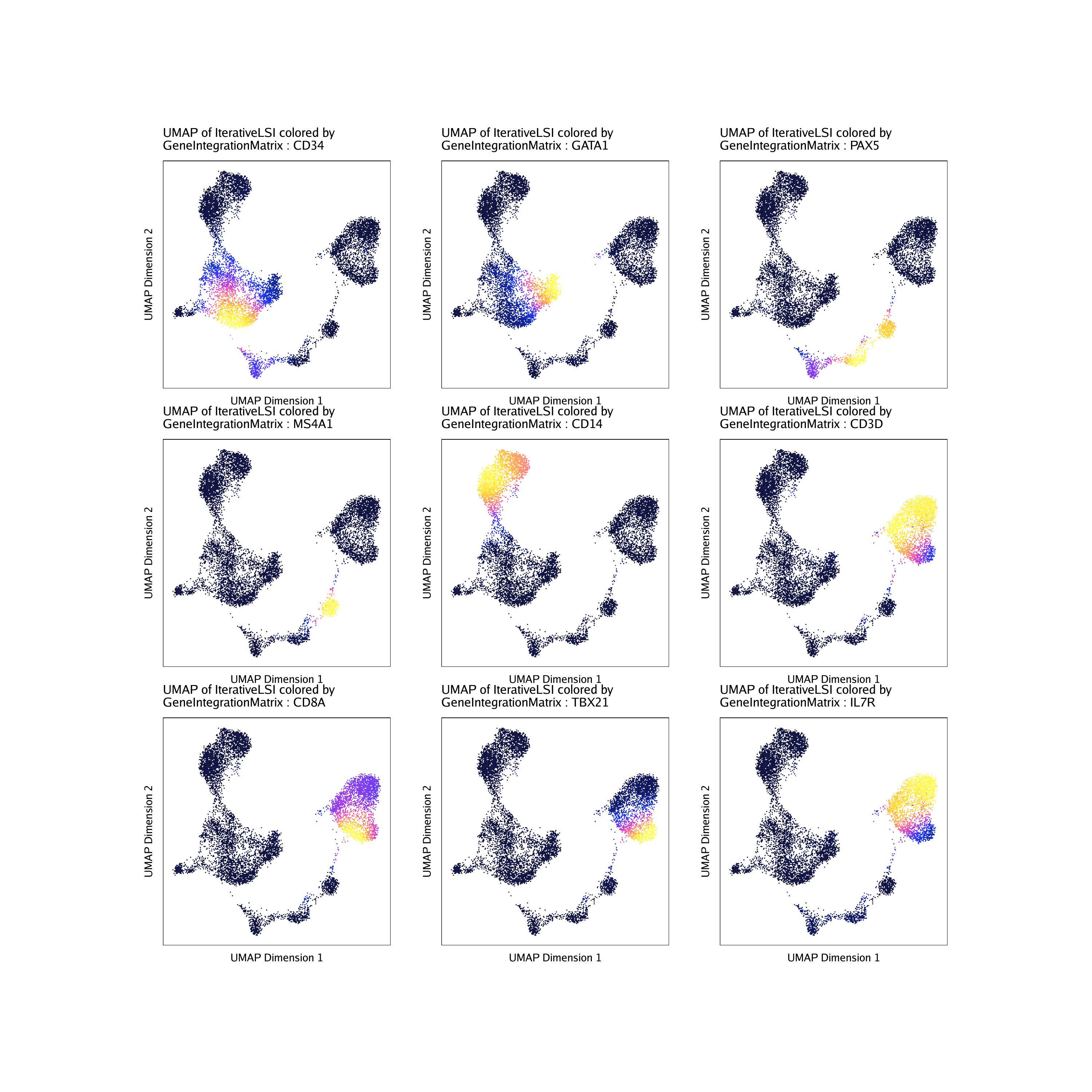
Now, lets make some UMAP plots overlayed with the gene expression values from our GeneIntegrationMatrix.
markerGenes  <- c(
    "CD34", #Early Progenitor
    "GATA1", #Erythroid
    "PAX5", "MS4A1", #B-Cell Trajectory
    "CD14", #Monocytes
    "CD3D", "CD8A", "TBX21", "IL7R" #TCells
  )

p1 <- plotEmbedding(
    ArchRProj = projHeme3,
    colorBy = "GeneIntegrationMatrix",
    name = markerGenes,
    continuousSet = "horizonExtra",
    embedding = "UMAP",
    imputeWeights = getImputeWeights(projHeme3)
)
## Getting ImputeWeights
## ArchR logging to : ArchRLogs/ArchR-plotEmbedding-f66370e499ac-Date-2020-04-15_Time-10-20-59.log
## If there is an issue, please report to github with logFile!
## Getting UMAP Embedding
## ColorBy = GeneIntegrationMatrix
## Getting Matrix Values…
## Getting Matrix Values…
##
## Imputing Matrix
## Using weights on disk
## Using weights on disk
## Plotting Embedding
## 1 2 3 4 5 6 7 8 9
## ArchR logging successful to : ArchRLogs/ArchR-plotEmbedding-f66370e499ac-Date-2020-04-15_Time-10-20-59.log
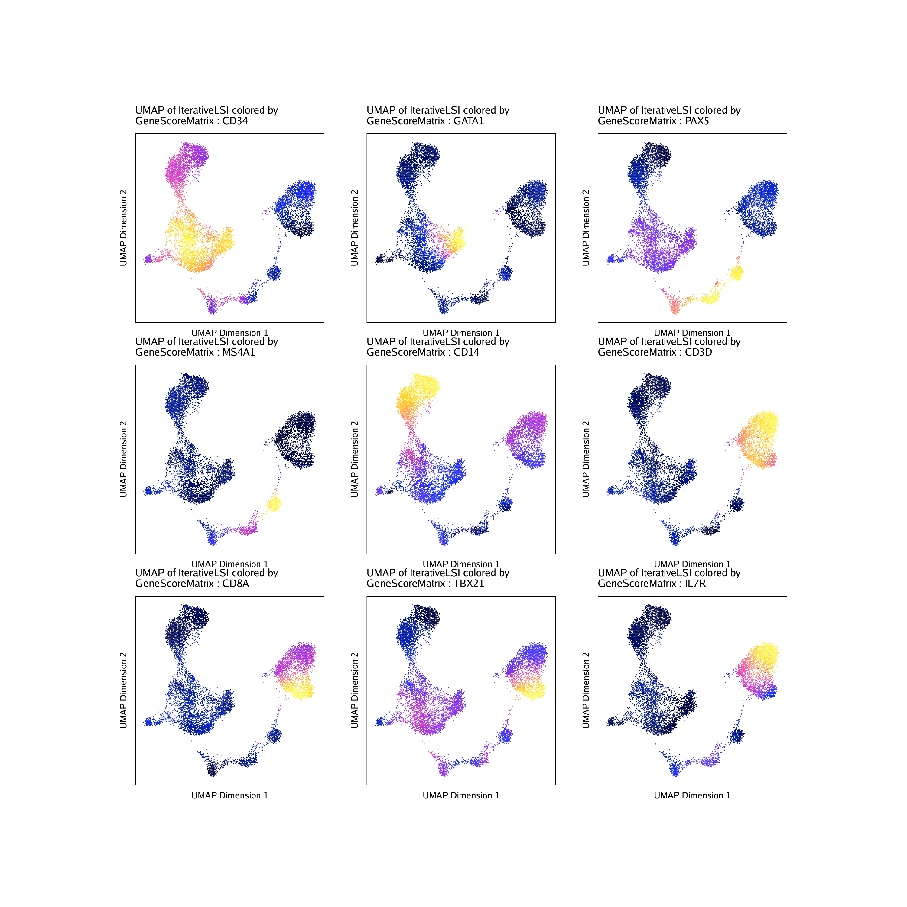
We can make the same UMAP plots but overlay them with the gene score values from our GeneScoreMatrix
p2 <- plotEmbedding(
    ArchRProj = projHeme3,
    colorBy = "GeneScoreMatrix",
    continuousSet = "horizonExtra",
    name = markerGenes,
    embedding = "UMAP",
    imputeWeights = getImputeWeights(projHeme3)
)
## Getting ImputeWeights
## ArchR logging to : ArchRLogs/ArchR-plotEmbedding-f6632d4259ce-Date-2020-04-15_Time-10-21-15.log
## If there is an issue, please report to github with logFile!
## Getting UMAP Embedding
## ColorBy = GeneScoreMatrix
## Getting Matrix Values…
## Getting Matrix Values…
##
## Imputing Matrix
## Using weights on disk
## Using weights on disk
## Plotting Embedding
## 1 2 3 4 5 6 7 8 9
## ArchR logging successful to : ArchRLogs/ArchR-plotEmbedding-f6632d4259ce-Date-2020-04-15_Time-10-21-15.log
To plot all marker genes we can use cowplot
p1c <- lapply(p1, function(x){
    x + guides(color = FALSE, fill = FALSE) +
    theme_ArchR(baseSize = 6.5) +
    theme(plot.margin = unit(c(0, 0, 0, 0), "cm")) +
    theme(
        axis.text.x=element_blank(),
        axis.ticks.x=element_blank(),
        axis.text.y=element_blank(),
        axis.ticks.y=element_blank()
    )
})

p2c <- lapply(p2, function(x){
    x + guides(color = FALSE, fill = FALSE) +
    theme_ArchR(baseSize = 6.5) +
    theme(plot.margin = unit(c(0, 0, 0, 0), "cm")) +
    theme(
        axis.text.x=element_blank(),
        axis.ticks.x=element_blank(),
        axis.text.y=element_blank(),
        axis.ticks.y=element_blank()
    )
})

do.call(cowplot::plot_grid, c(list(ncol = 3), p1c))

As expected, the results from these two methods for inferring gene expression are similar but not identical.
To save an editable vectorized version of this plot, we use the plotPDF() function.
plotPDF(plotList = p1,
    name = "Plot-UMAP-Marker-Genes-RNA-W-Imputation.pdf",
    ArchRProj = projHeme3,
    addDOC = FALSE, width = 5, height = 5)
## [1] “plotting ggplot!”
## [1] “plotting ggplot!”
## [1] “plotting ggplot!”
## [1] “plotting ggplot!”
## [1] “plotting ggplot!”
## [1] “plotting ggplot!”
## [1] “plotting ggplot!”
## [1] “plotting ggplot!”
## [1] “plotting ggplot!”
## [1] 0